Author

Date Manipulations in JavaScript Using Moment-Timezone

by admin-postApril 11, 2020no comment

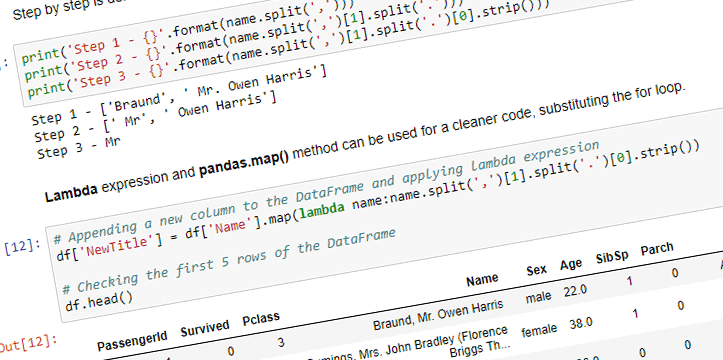
Recently, I was working on some GraphQL data fetching tutorial. The fetched data included time in Unix time format. The author proceeded with 10 minutes writing, in my opinion, unnecessary datetime processing function, to simply display the date output in the certain string format. The function would convert the timestamp to new Date(), extract year, month (which was also converted to display month name based on the corresponding number), date, hour, etc. as variables, and then finally, display it using template literals. The author also used "86400" seconds in adding dates (24 hours, 60 minutes, 60 seconds).

In my experience with Unix time, or in particular Timestamps used in Google Firestore, it is better to avoid writing these type of functions, especially, while dealing with time sensitive data, operations like addition and subtraction of time periods, or dealing with the timezones and daylight saving times.

There are libraries available, like moment-timezone, that make this type of operations easy, and reduce the chance of introducing unnecessary bugs.

Python,

Plotting Error Bars in Python using Matplotlib and Numpy Random

by admin-postMarch 17, 2018no comment

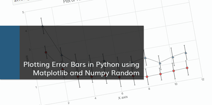
A friend of mine needed help with plotting clusters with corresponding asymmetrical error bars. I decided to write a blog post about plotting error bars in Python after helping with the problem. The notebook can be also viewed on Github.

Error Bars

Error bars are graphical representations of the error or uncertainty in data, and they assist correct interpretation. For scientific purposes, reporting of errors is crucial in understanding the given data. Mostly error bars represent range and standard deviation of a dataset. They can help visualize how the data is spread around the mean value.

The Data

The data shown below is randomly generated for plotting purposes. This blog post is not about correct statistical interpretation of error bars, and solely written for demonstration purposes.

We will be using numpy for data generation. Let’s start by importing numpy.

In [1]:

# Importing numpy
import numpy as np
np.__version__

Out[1]:

'1.14.0'

Deep Learning, Python,

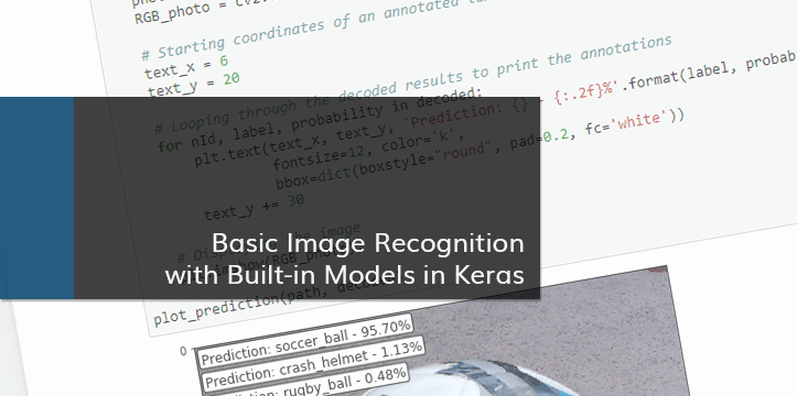
Basic Image Recognition with Built-in Models in Keras

by admin-postMarch 13, 2018no comment

In this blog post we are going to look at Image Recognition with built-in models available in Keras. The notebook can be also viewed on Github.

There are various pre-trained models available in Keras. The weights for these models are trained on a subset of ImageNet dataset. ImageNet is an image dataset containing millions of images with each image described in words. The models are trained on a dataset of 1000 types of common objects (the list of 1000 categories). This dataset is used during The ImageNet Large Scale Visual Recognition Challenge (ILSVRC).

The models for image classification available in Keras are listed below:

Xception
VGG16
VGG19
ResNet50
InceptionV3
InceptionResNetV2
MobileNet
DenseNet
NASNet

Once the model is instantiated, the weights are automatically downloaded to ~/.keras/models/ folder. We will be implementing ResNet50 (50 Layer Residual Network – further reading: Deep Residual Learning for Image Recognition) in the example below. The file containing weights for ResNet50 is about 100MB.

The versions

In this example I am using Keras v.2.1.4 and TensorFlow v.1.5.0 with GPU (using NVIDIA CUDA).

Books,

Reading – February 2018

by admin-postMarch 6, 2018no comment

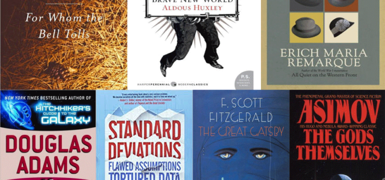
This is a summary of non-Computer Science related books I’ve completed in February. As you may remember, at the beginning of this year I decided to increase my reading, with a goal of reading minimum 50 pages a day.

For February, I’ve read 1672 pages, with the average 60 pages/day, and completed 7 books. My best day was 113 pages, while my worst was about 20 pages during February.

For 2018, so far I’ve read 3615 pages, with the average 61 pages/day, and completed 15 books.

Reading – January 2018

Below is the list of books I’ve completed in February:

Deep Learning, Machine Learning, Python,

Basic Example of a Neural Network with TensorFlow and Keras

by admin-postMarch 6, 2018no comment

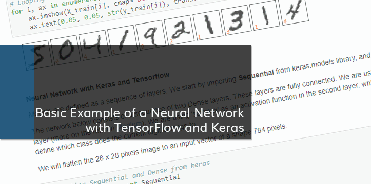
This blog post covers basic example of a Neural Network, using TensorFlow and Keras in Python. The notebook can be also viewed on Github.

TensorFlow and Keras

TensorFlow was developed at Google to use internally for machine learning tasks, and applied to the applications like speech recognition, Search, Gmail, etc. It was made public in 2015 as an open source application. The library is in C++, used with Python API. TensorFlow can be used for various problems like image recognition, language processing, implementation in self-driving cars, etc. There are various alternatives available to TensorFlow such as Theano, and Torch.

We are going to use Keras in this notebook, with Tensorflow as a backend engine. Keras is a high-level wrapper, which can be used both with TensorFlow and Theano. It simplifies common operations. The code is similar to scikit-learn, making it easier to get used to it, while in the background TensorFlow or Theano is used for processing.

The data

In this example we will be looking at MNIST database (a subset of a larger set by National Institute of Standards and Technology). This is a classic dataset containing 60000 training images, 10000 test images, and corresponding training and test labels. The images are handwritten digits, in the shape of 28 x 28 pixels, and divided into 10 categories (from 0 to 9).

The versions

In this example I am using Keras v.2.1.4 and TensorFlow v.1.5.0 with GPU (using NVIDIA CUDA). Running examples on a GPU can speed up the training process.

In [1]:

# To avoid warnings
import warnings
warnings.filterwarnings('ignore')

# Importing keras and tensorflow, and printing the versions
import keras
print('Keras: {}'.format(keras.__version__))

import tensorflow as tf
print('TensorFlow: {}'.format(tf.__version__))

Using TensorFlow backend.

Keras: 2.1.4
TensorFlow: 1.5.0

Python,

Pandas – Tips and Tricks – df.loc, df.iloc

by admin-postFebruary 27, 2018no comment

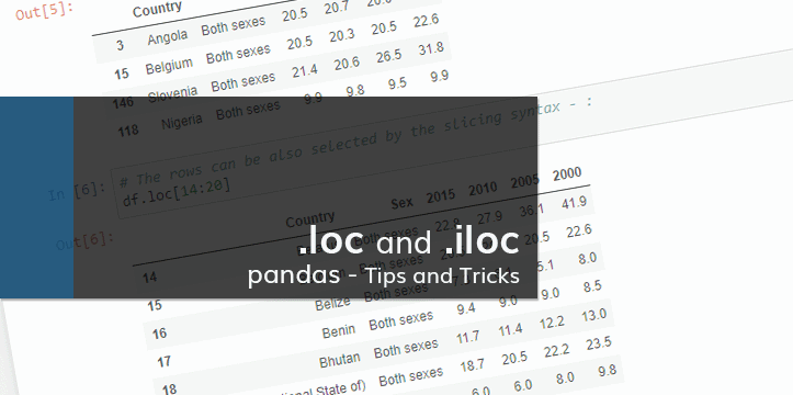
This notebook is a part of Pandas – Tips and Tricks mini-series, focusing on different aspects of pandas library in Python. In the below examples we will be looking at selecting the data by using .loc and .iloc methods. The notebook is also available on GitHub.

.loc: is primarily label based indexing.

.iloc: is primarily integer position based indexing.

Previous blog posts on the topic: Data import with Python, using pandas DataFrame – Part 1

Let’s start by importing pandas and loading the data:

In [1]:

# Loading the library
import pandas as pd

# I am using the data from WHO as an example
df = pd.read_csv('Data/SuicBoth.csv')

# Checking the DataFrame shape
print(df.shape)

# Checking the imported data
df.head()

(183, 6)

Machine Learning, Python,

Statistical Terms in Data Science and Regression Metrics

by admin-postFebruary 14, 2018no comment

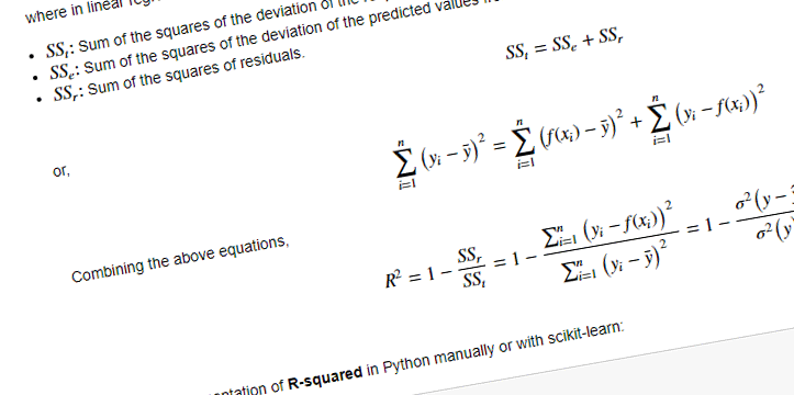
Various statistical concepts are incorporated in Data Science. In this notebook I am going to cover some basic statistical terms, and talk about metrics used in Data Science for Regression tasks. This notebook can be also viewed on Github.

1. Statistical terms

Let’s look at some simple statistical terms in detail:

Mean ( $\bar{x}$ ): Averaging. Mean is a sum of all values divided by the number of values:

$\bar{x} = \frac{\sum_{i=1}^{n}x_i}{n}$

Variance ( $\sigma^2$ ): Describes the spread of a distribution. For a set of values, the variance:

$\sigma^2 = \frac{1}{n}\sum_{i=1}^{n}\big(x_i - \bar{x}\big)^2$

Standard Deviation ( $\sigma$ ): Square root of variance, is in the units of the data it represents:

$\sigma = \sqrt{\frac{1}{n}\sum_{i=1}^{n}\big(x_i - \bar{x}\big)^2}$

Books,

Reading – January 2018

by admin-postFebruary 2, 2018no comment

We live in the interesting times. The information is available to us through various media. Yes, we are bombarded by the information, and the noise can suppress the valuable bits of it. But it is still there, available for us (as conscious beings, as humans) to absorb it in our limited lifespan.

Getting closer to the end of the 2017, the idea of limited time had sunk in me. Being present here, on a habitable planet, in a solar system, in some corner of the galaxy, in some part of the universe, made me appreciate the time we were given. Let’s call it a resolution (not my favorite word), while my brain functions I decided to learn something new every day.

I decided to increase my reading. To be honest, I was never a fan of reading. I was too picky in the selection of the topics. Growing up, I was more interested in history and science related books rather than fiction. I would generally spend a month or two over a book. In the last couple years I’ve been intensively reading various Computer Science related books (e.g., topics like Python, Data Science, Algorithms, etc.) on a laptop screen. Now I am capable of reading the books on an iPad or on my phone without much discomfort. Compared to the paperback, I am even more productive with the electronic versions of the books. I’ve set a goal of reading minimum 50 pages a day of not CS / IT related books. To be realistic, it wasn’t always possible to meet the goal (life happens). My best day was 219 pages, while my worst was about 10 pages. In January I’ve read 1943 pages, with the average 63 pages/day, and completed 8 books.

Below is the list of books I’ve completed in January:

Python,

String, String Methods, and String Manipulation

by admin-postJanuary 30, 2018no comment

String is a collection of characters. Any character can be accessed by its index. The indexing of a string starts at 0 (or -1 if it’s indexed from the end). We can get the number of characters in a string by using built-in function len. Compared to the indexing, len is not zero based.

In [1]:

# Creating a string
text = 'Some collection of words'

# Assigning the number of characters in the given string to a variable
total_char = len(text)

# Printing the total number of characters
print('Number of characters = {}'.format(total_char))

Number of characters = 24

Machine Learning, Python,

Machine Learning – Programming Exercise 2: Logistic Regression

by admin-postOctober 11, 2017no comment

Programming Exercise 2: Logistic Regression

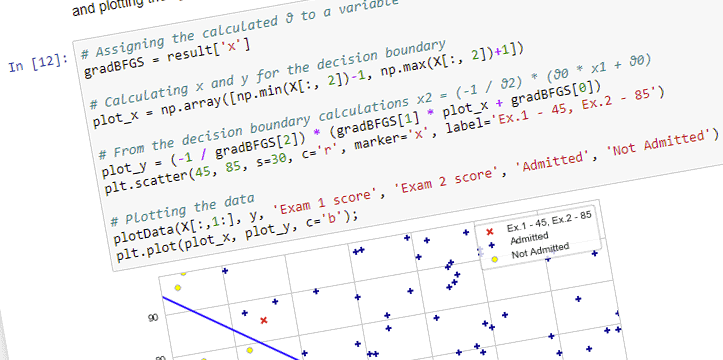
The following blog post contains exercise solution for logistic regression assignment from the Machine Learning course by Andrew Ng. Also, this blog post is available as a jupyter notebook on GitHub.

In [1]:

# Standard imports. Importing seaborn for styling.
%matplotlib inline
import numpy as np
import matplotlib.pyplot as plt
import seaborn; seaborn.set_style('whitegrid')

Older Posts

codeWithMax

codeWithMax

Author

Date Manipulations in JavaScript Using Moment-Timezone

Plotting Error Bars in Python using Matplotlib and Numpy Random

Error Bars

The Data

Basic Image Recognition with Built-in Models in Keras

The versions

Reading – February 2018

Basic Example of a Neural Network with TensorFlow and Keras

TensorFlow and Keras

The data

The versions

Pandas – Tips and Tricks – df.loc, df.iloc

Statistical Terms in Data Science and Regression Metrics

1. Statistical terms

Reading – January 2018

String, String Methods, and String Manipulation

Machine Learning – Programming Exercise 2: Logistic Regression

Programming Exercise 2: Logistic Regression