Various statistical concepts are incorporated in Data Science. In this notebook I am going to cover some basic statistical terms, and talk about metrics used in Data Science for Regression tasks. This notebook can be also viewed on Github.
1. Statistical terms
Let’s look at some simple statistical terms in detail:
Mean (

Variance (
^2")
Standard Deviation (
^2}")
Note: If the data is a subset of the entire population, the denominator (n) in the variance and standard deviation calculations becomes (n-1).
Note 2:
- Predictor (X) is also called feature, or input variable
- Response (y) is also called target, output variable, or label
We are going to create an array using numpy, define methods for manual calculation of the above terms, and then implement built in numpy functions:
# Importing numpy library
import numpy as np

# Creating an array
x = np.array([3, 8, 5, 6, 2])
# Defining a method calculating the mean of a given array
def mean_calc(num):
    # Using max(len(num), 1) to avoid division by 0 for empty arrays.
    return float(sum(num)) / max(len(num), 1)

# Defining a method calculating the variance of a given array
def var_calc(num):
    x_bar = mean_calc(num)
    return sum(abs(num - x_bar)**2) / max(len(num), 1)

# Defining a method calculating the standard deviation of a given array
def std_calc(num):
    return var_calc(num)**(0.5)

# Printing calculated values
print('For a given array {}:'.format(x))
print('Mean: {0:15.3f}'.format(mean_calc(x)))
print('Variance: {0:11.3f}'.format(var_calc(x)))
print('Std. Deviation: {0:2.3f}'.format(std_calc(x)))
# Or with built-in numpy methods:
print('For a given array {}:'.format(x))
print('Mean: {0:15.3f}'.format(float(x.mean())))
print('Variance: {0:11.3f}'.format(x.var()))
print('Std. Deviation: {0:2.3f}'.format(x.std()))
2. Metrics
There are different ways available for measuring model performance, and they are well incorporated in sckit-learn.metrics. Before we get to the metrics, let’s look at one more statistical term:
Residuals: Deviation of predicted values from actual. For the linear model, it is the vertical deviation from the line.
2.1. Regression Metrics
Below are the most common metrics used to measure regression performance:
2.1.1. R-squared (coefficient of determination)
R-squared measures how response variables predicted by the model are fitting the actual values. For a linear model the values are in the range of 0 to 1. The R-squared value of 1 indicates that the regression line perfectly fits the data, there is no error using this model.
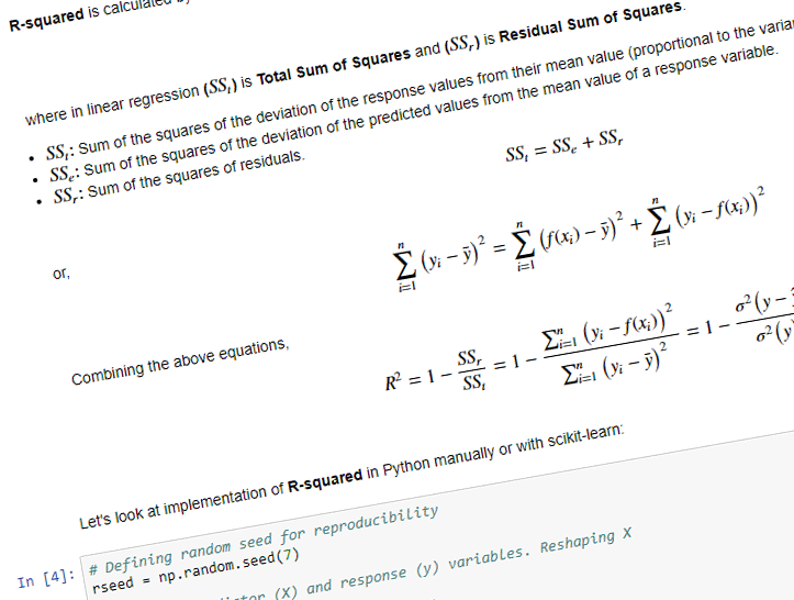
R-squared is calculated by the below equation,

where in linear regression (

: Sum of the squares of the deviation of the predicted values from the mean value of a response variable.

or,
^2 = \sum_{i=1}^{n}\big(f(x_i) - \bar{y}\big)^2 + \sum_{i=1}^{n}\big(y_i - f(x_i)\big)^2")
Combining the above equations,
\big)^2}{\sum_{i=1}^{n}\big( y_i - \bar{y}\big)^2} = 1 - \frac {\sigma{^2}\big(y - \hat{y}\big)}{\sigma{^2}\big(y\big)}")
Let’s look at implementation of R-squared in Python manually or with scikit-learn:
# Defining random seed for reproducibility
rseed = np.random.seed(7)

# Defining predictor (X) and response (y) variables. Reshaping X
X = np.arange(12, 22)
y = X * 10 + np.random.rand(len(X)) * 20

# Reshaping X array to a column vector
X = X[:, np.newaxis]

# Checking the shapes of X and y
print(X.shape, y.shape)
# Importing Linear Regression
from sklearn.linear_model import LinearRegression

# Creating linear regression object
model = LinearRegression()

# Fitting the data to the model and constructing the best fit line
model.fit(X, y)

# We can check the slope and intercept of the line
print('Slope:   {0:10.3f}\nIntercept:  {1:7.3f}'.format(model.coef_[0], model.intercept_))
# Importing matplotlib for plotting, and seaborn for styling
%matplotlib inline
import matplotlib.pyplot as plt
import seaborn as sns; sns.set_style('whitegrid')
# Let's calculate the response variable predicted by the model.
# It can be done by: y_pred = X * model.coef_[0] + model.intercept_
# or by using model.predict function from scikit-learn
y_pred = model.predict(X)
# We also need to plot the model line
x_fit = np.linspace(10, 24)
y_fit = model.predict(x_fit[:, np.newaxis])
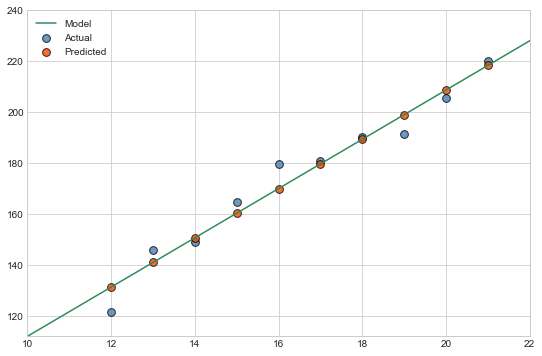
# Plotting the Actual values, Predicted values, and Model fit
fig, ax = plt.subplots(figsize=(9, 6))
ax.scatter(X, y, s=60, c='steelblue', alpha=0.8, edgecolors='k', label='Actual')
ax.scatter(X, y_pred, s=60, c='orangered', alpha=0.8, edgecolors='k', label='Predicted')
ax.plot(x_fit, y_fit, c='seagreen', label='Model')
ax.set_xlim(x_fit.min(), x_fit.max() - 2)
ax.set_ylim(y_fit.min(), 240)
plt.legend();
# Manually calculating the R-squared
r_squared = 1 - (np.sum((y - y_pred)**2) / np.sum((y - y.mean())**2))
print('R-squared(manual):       {0:7.4f}'.format(r_squared))

# R-squared with variance equation
r_sq_var = 1 - (y - y_pred).var() / y.var()
print('R-squared(variance):     {0:7.4f}'.format(r_sq_var))

# Or using scikit-learns r2_score
from sklearn.metrics import r2_score
print('R-squared(scikit-learn): {0:7.4f}'.format(r2_score(y, y_pred)))
2.1.2. Mean Absolute Error (MAE)
MAE is the sum of the absolute values of the residuals divided by the number of values, hence the name mean absolute error. MAE gives the idea of the magnitude of the error. The MAE value of 0 indicates that the regression line perfectly fits the data, there is no error using this model.
MAE is calculated by the below equation,
\big|}{n}")
# Manually calculating the MAE
mae = np.abs(y - y_pred).mean()
print('MAE(manual):       {0:7.4f}'.format(mae))

# Or using scikit-learns mean_absolute_error
from sklearn.metrics import mean_absolute_error
mean_absolute_error(y, y_pred)
print('MAE(scikit-learn): {0:7.4f}'.format(mean_absolute_error(y, y_pred)))
2.1.3. Mean Squared Error (MSE)
MSE is the sum of the squares of residuals divided by the number of values, hence the name mean squared error. Like MAE, MSE gives the idea of the magnitude of the error. Root Mean Squared Error (RMSE) is the squared root of MSE, converting the units back to the original units of the response variable.
MSE is calculated by the below equation,
\big)^2}{n}")
# Manually calculating the MSE
mse = ((y - y_pred)**2).mean()
print('MSE(manual):       {0:7.4f}'.format(mse))

# Or using scikit-learns mean_squared_error
from sklearn.metrics import mean_squared_error
mean_absolute_error(y, y_pred)
print('MSE(scikit-learn): {0:7.4f}'.format(mean_squared_error(y, y_pred)))