Programming Exercise 2: Logistic Regression
The following blog post contains exercise solution for logistic regression assignment from the Machine Learning course by Andrew Ng. Also, this blog post is available as a jupyter notebook on GitHub.
# Standard imports. Importing seaborn for styling.
%matplotlib inline
import numpy as np
import matplotlib.pyplot as plt
import seaborn; seaborn.set_style('whitegrid')
1 Logistic Regression
The task for this exercise is to build a logistic regression model that estimates an applicant’s probability of admission based on the scores from two exams.
1.1 Visualizing the data
We start by importing and plotting the given data:
# Loading the data. The first two columns contain the exam scores and the third column contains the label.
data = np.loadtxt('data/ex2data1.txt', delimiter=',')
X, y = data[:,:2], data[:,2]

# Viewing the imported values (first 5 rows)
X[:5], y[:5]
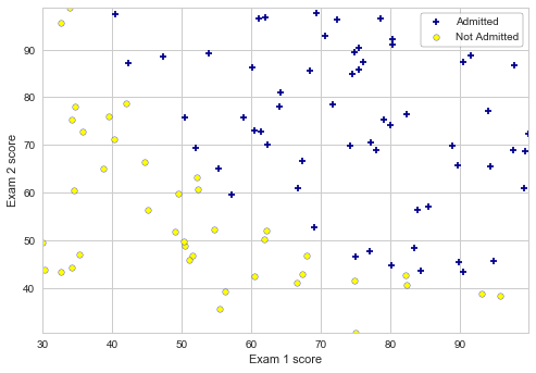
# Creating plotData method to display the figure where the axes are the two exam scores.
def plotData(x, y, xlabel, ylabel, labelPos, labelNeg):

    # Separating positive and negative scores (in this case 1 and 0 values):
    pos = y==1
    neg = y==0

    # Scatter plotting the data, filtering them according the pos/neg values:
    plt.scatter(x[pos, 0], x[pos, 1], s=30, c='darkblue', marker='+', label=labelPos)
    plt.scatter(x[neg, 0], x[neg, 1], s=30, c='yellow', marker='o', edgecolors='b', label=labelNeg)

    # Labels and limits:
    plt.xlabel(xlabel)
    plt.ylabel(ylabel)
    plt.xlim(x[:, 0].min(), x[:, 0].max())
    plt.ylim(x[:, 1].min(), x[:, 1].max())

    # Legend:
    pst = plt.legend(loc='upper right', frameon=True)
    pst.get_frame().set_edgecolor('k');
# Plotting the initial figure:
plotData(X, y, 'Exam 1 score', 'Exam 2 score', 'Admitted', 'Not Admitted')
1.2 Implementation
1.2.1 Warmup exercise: sigmoid function
Logistic regression hypothesis is defined as
![]() ,
,
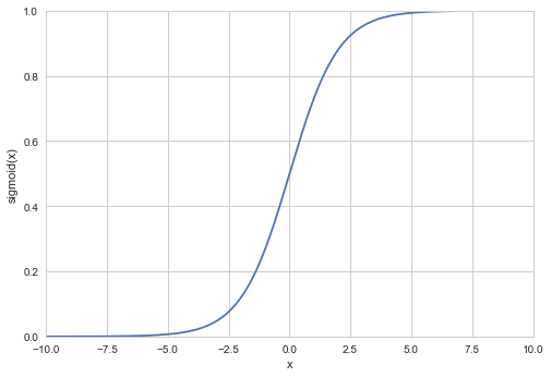
where g is the sigmoid function. The sigmoid function is defined as
![]()
# While using (return 1 / (1 + np.exp(-z))), per the sigmoid function, I was getting an overflow warning.
# As a solution warning can be ignored, or the dtype can be changed to not cause the error/warning.
# I used expit method from scipy to eliminate this issue.
from scipy.special import expit

# Defining sigmoid function:
def sigmoid(z):
    # return 1 / (1 + np.exp(-z))
    return expit(z)
# Calculating,
x_val = np.linspace(-10, 10, 10000)

# and plotting the calculated sigmoid function:
plt.plot(x_val, sigmoid(x_val))

# Labels and limits
plt.xlabel('x')
plt.ylabel('sigmoid(x)')
plt.xlim(x_val.min(), x_val.max())
plt.ylim(0, 1);
1.2.2 Cost function and gradient
In this part of the assignment we will implement cost function and gradient methods for logistic regression.
# Defining costFunction method:
def costFunction(theta, X, y):
    # Number of training examples
    m = len(y)

    # eps = 1e-15  was taken from the solution by jellis18
    # https://github.com/jellis18/ML-Course-Solutions/blob/master/ex2/ex2.ipynb
    # It is tolerance for sigmoid function, fixes loss of precision error.
    # Eliminates errors while using BFGS minimization in calculations using scipy.
    eps = 1e-15

    hThetaX = sigmoid(np.dot(X, theta))

    J = - (np.dot(y, np.log(hThetaX)) + np.dot((1 - y), np.log(1 - hThetaX + eps))) / m

    return J
# Defining gradientFunc:
def gradientFunc(theta, X, y):
    # Number of training examples
    m = len(y)

    hThetaX = sigmoid(np.dot(X, theta))

    gradient =  np.dot(X.T, (hThetaX - y)) / m

    return gradient
We add an additional first column to X and set it to all ones. Also, we add theta and initialize the parameters to 0’s.
X = np.hstack((np.ones((X.shape[0],1)), X))

theta = np.zeros(X.shape[1])
theta
We call costFunction and gradientFunc methods using the initial parameters of θ.
J = costFunction(theta, X, y)
gradient = gradientFunc(theta, X, y)

# We should see that the cost is about 0.693 per the exercise:
print("Cost: %0.3f"%(J))
print("Gradient: {0}".format(gradient))
1.2.3 Learning parameters with scipy.optimize using .minimize
scipy.optimize.minimize uses BFGS as a default method for the function minimum calculations of unconstrained function, and finds the best parameters for θ (in our case logistic regression cost function). We are feeding objective (cost) function, x0 (initial guess), arguments, and Jacobian (gradient) of objective function to the algorithm.
# Importing minimize from scipy:
from scipy.optimize import minimize

# Finding the best parameters for θ, using the methods we created earlier:
# Expecting to see the cost around 0.203 per the assignment.
result = minimize(costFunction, theta, args=(X,y), method='BFGS', jac=gradientFunc, options={'maxiter' : 400, 'disp': True})
result
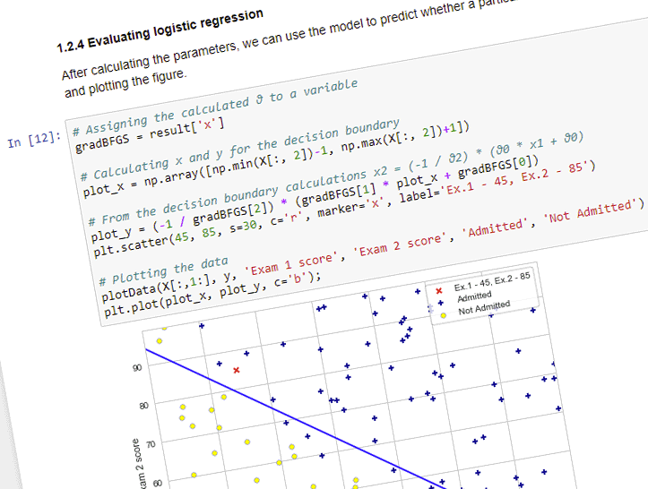
1.2.4 Evaluating logistic regression
After calculating the parameters, we can use the model to predict whether a particular student will be admitted. We are also calculating the decision boundary, and plotting the figure.
# Assigning the calculated θ to a variable
gradBFGS = result['x']

# Calculating x and y for the decision boundary
plot_x = np.array([np.min(X[:, 2])-1, np.max(X[:, 2])+1])

# From the decision boundary calculations x2 = (-1 / θ2) * (θ0 * x1 + θ0)
plot_y = (-1 / gradBFGS[2]) * (gradBFGS[1] * plot_x + gradBFGS[0])
plt.scatter(45, 85, s=30, c='r', marker='x', label='Ex.1 - 45, Ex.2 - 85')

# Plotting the data
plotData(X[:,1:], y, 'Exam 1 score', 'Exam 2 score', 'Admitted', 'Not Admitted')
plt.plot(plot_x, plot_y, c='b');
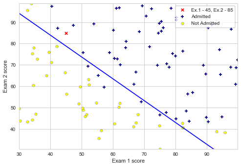
# For a student with an Exam 1 score of 45 and an Exam 2 score of 85, you should expect
# to see an admission probability of 0.776
probability = sigmoid(np.dot(gradBFGS, np.array([1, 45.,85.])))

print("Exam scores: 45 and 85")
print("Probability of acceptance: %0.3f"%(probability))
Next step is to calculate the training accuracy of the classifier by computing the percentage of examples it got correct:
def predict(theta, X):
    hThetaX = sigmoid(np.dot(X, theta))

    arr = []
    for h in hThetaX:
        if (h > 0.5):
            arr.append(1)
        else:
            arr.append(0)

    return np.array(arr)

# Prediction using calculated values of θ and given data set
p = predict(gradBFGS, X)

# Training accuracy
print('Training Accuracy of the classifier: {0}%'.format(np.sum(p==y) / p.size * 100))
2 Regularized logistic regression
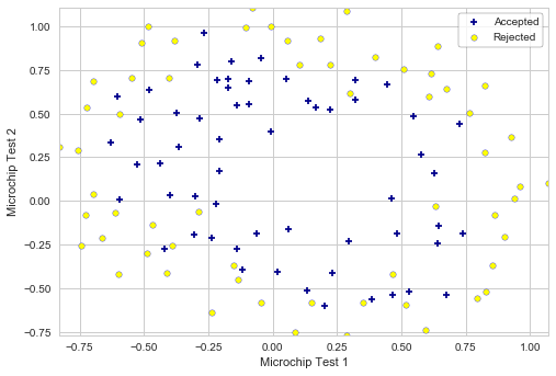
In this part of the exercise, regularized logistic regression is implemented to predict whether microchips from a fabrication plant passes quality assurance (QA).
2.1 Visualizing the data
We start by importing the data and visualizing it, as in the previous part of the exercise.
data = np.loadtxt('data/ex2data2.txt', delimiter=',')
X, y = data[:,:2], data[:,2]

# Viewing the imported values (first 5 rows)
X[:5], y[:5]
Plotting the imported data:
plotData(X, y, 'Microchip Test 1', 'Microchip Test 2', 'Accepted', 'Rejected')
2.2 Feature mapping
One way to fit the data better is to create more features from each data point. To do that we can use PolynomialFeatures from the scikit-learn library to map the features into all polynomial terms of x1 and x2, up to the sixth power for the current exercise.
# Importing PolynomialFeatures
from sklearn.preprocessing import PolynomialFeatures

# Creating the model
poly = PolynomialFeatures(6)

# Transforming the data into the sixth power polynomial
X2 = poly.fit_transform(X)
X2.shape
2.3 Cost function and gradient
Cost function and gradient methods for regularized logistic regression.
# Defining regularized costFunction method:
def costFunctionR(theta, X, y, lam):
    # Number of training examples
    m = len(y)

    eps = 1e-15

    hThetaX = sigmoid(np.dot(X, theta))

    J = - (np.dot(y, np.log(hThetaX)) + np.dot((1 - y), np.log(1 - hThetaX + eps)) -
           1/2 * lam * np.sum(np.square(theta[1:]))) / m

    return J
# Defining regularized gradientFunc:
def gradientFuncR(theta, X, y, lam):
    # Number of training examples
    m = len(y)

    hThetaX = sigmoid(np.dot(X, theta))

    # We're not regularizing the parameter θ0, replacing it with 0
    thetaNoZeroReg = np.insert(theta[1:], 0, 0)

    gradient =  (np.dot(X.T, (hThetaX - y)) + lam * thetaNoZeroReg) / m

    return gradient
# We add theta and initialize the parameters to 0's.
initial_theta = np.zeros(X2.shape[1])
initial_theta
We call costFunctionR and gradientFuncR methods using the initial parameters of θ.
J = costFunctionR(initial_theta, X2, y, 1)
gradient = gradientFuncR(initial_theta, X2, y, 1)

# We should see that the cost is about 0.693 per the exercise:
print("Cost: %0.3f"%(J))
print("Gradient: {0}".format(gradient))
Calculating the parameters with scipy.optimize using *.minimize, as in exercise part 1.2.3.
result2 = minimize(costFunctionR, initial_theta, args=(X2, y, 1), method='BFGS', jac=gradientFuncR,
                   options={'maxiter' : 400, 'disp': False})
result2['x']
2.4 Plotting the decision boundary
The decision boundary function is provided with the exercise file. I am using the decision boundary calculations similar to the ones provided in scikit-learn examples. In this case, we define the data used for meshgrid calculation, and then plot the contour plot using the meshgrid data.
def plotDecisionBoundary(X, y, title):
    # Plot the data
    plotData(X[:, 1:3], y, 'Microchip Test 1', 'Microchip Test 2', 'Accepted', 'Rejected')

    # Defining the data to use in the meshgrid calculation. Outputting xx and yy ndarrays
    x_min, x_max = X[:, 1].min() - 1, X[:, 1].max() + 1
    y_min, y_max = X[:, 2].min() - 1, X[:, 2].max() + 1
    xx, yy = np.meshgrid(np.arange(x_min, x_max, 0.02), np.arange(y_min, y_max, 0.02))

    Z = sigmoid(poly.fit_transform(np.c_[xx.ravel(), yy.ravel()]).dot(result2['x']))
    Z = Z.reshape(xx.shape)

    # Plotting the contour plot
    plt.contour(xx, yy, Z, [0.5], linewidths=1, colors='g')
    plt.title(title)
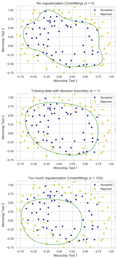
2.5 Optional (ungraded) exercises
In this part of exercise we will get to try different regularization parameters. We are observing overfitting with low λ values. With the larger λ values, we observe the decision boundary not following the data well, thus underfitting the data.
plt.figure(figsize=(6, 15))
plt.subplots_adjust(hspace=0.3)

# Creating 3 subplots using 3 different λ values
for i, lam in enumerate([0, 1, 100]):
    result2 = minimize(costFunctionR, initial_theta, args=(X2, y, lam), method='BFGS', jac=gradientFuncR,
                       options={'maxiter' : 400, 'disp': False})

    if (lam == 0):
        title = 'No regularization (Overfitting) (λ = 0)'
    elif (lam == 100):
        title = 'Too much regularization (Underfitting) (λ = 100)'
    else:
        title = 'Training data with decision boundary (λ = 1)'

    plt.subplot(3, 1, i+1)

    # Plotting the decision boundary plot
    plotDecisionBoundary(X2, y, title);
Downloadable content:
ex2data1.txt
ex2data2.txt